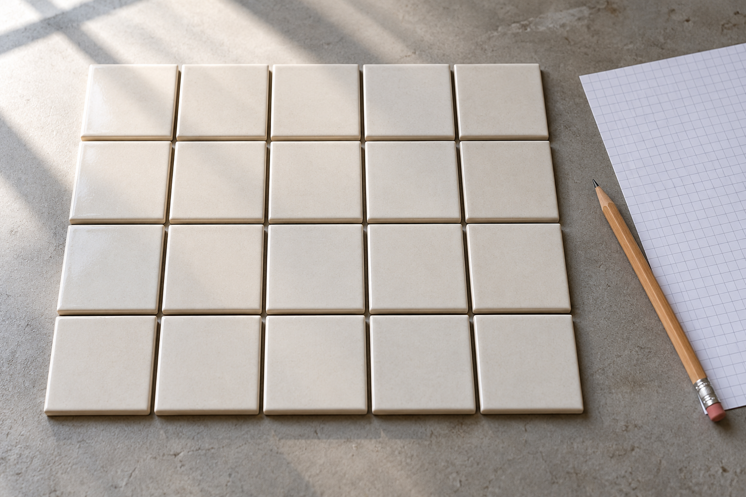
A box contains twenty inspected tiles and no cracks. It is easy to write “zero percent defective” on the inspection sheet. That describes the twenty tiles. It says less about every tile the factory has made. A confidence interval is meant to bridge that distance, but the number printed beside the estimate is only as trustworthy as the route used to get there.
Suppose the twenty tiles were chosen at random from a much larger run, and each tile could be classified clearly as cracked or uncracked. Those are assumptions for an example, not a report of a real inspection. A common shortcut for a proportion takes the observed fraction, estimates its standard error from that same fraction, and adds and subtracts a margin. With zero cracks, the estimated fraction is zero and the shortcut's estimated standard error is zero too. The resulting “95% interval” is zero to zero. The sample has produced apparent certainty precisely where it offers little.
The National Institute of Standards and Technology's guide to intervals for proportions calls this the normal-approximation method and warns against using it when an observed fraction is near zero or one. The problem is in the procedure, not in how neatly its endpoints are printed. A label saying 95% cannot rescue a calculation that behaves badly for the data at hand.
Where the percentage lives
The confidence level describes what happens if a sampling and calculation procedure is used again and again under its stated conditions. In the long run, a procedure with 95% coverage produces intervals containing the fixed population quantity about 95% of the time. For the one interval already calculated, the unknown quantity is either inside or outside it. NIST's explanation for intervals around a mean makes this distinction explicitly: the confidence coefficient attaches to the method, not to a fresh probability assigned to the particular finished interval.
This is the idea Jerzy Neyman formalized in his 1937 paper on statistical estimation. He treated the interval's endpoints as functions of a sample that has not yet been observed. The true population value stays fixed; different samples yield different endpoints. To know what a confidence claim means, one must know the sampling process, the quantity being estimated, and the rule for constructing those endpoints. The printed pair of numbers is the last step of that chain.
“95%” is also often a nominal target rather than an exact promise at every possible underlying proportion. Counts are discrete: in twenty trials, the number of cracks can only be zero, one, two, and so on. The actual chance that a particular formula covers the true proportion can jump as that proportion changes. Lawrence Brown, T. Tony Cai and Anirban DasGupta's 2001 comparison found persistently poor and erratic coverage for the simple interval often called the Wald interval. Their recommendation for small binomial samples included the older Wilson score interval, introduced in Edwin Wilson's 1927 paper. The methods are solving the same question with different rules, and their results need not agree.
For the hypothetical twenty tiles with no cracks, the two-sided Wilson calculation at a nominal 95% level gives an interval from zero to about 16%. Its upper end is not a prediction that sixteen percent of the run is defective. It expresses how high an underlying defect rate remains compatible with this small clean sample by that method. The zero-to-zero shortcut has erased that uncertainty. The arithmetic for the Wilson upper end here is about 3.84 divided by 20 plus 3.84, using the familiar 1.96 multiplier squared; NIST publishes the full Wilson formula. A different well-justified interval method may give a different upper bound. Naming the method is part of reporting the result.
The sample makes a second promise
Even a sound interval formula cannot repair a misleading sample. If someone takes twenty tiles only from the top of the nearest pallet, the calculation may measure variation among easily reached tiles while missing a problem in another shift or at the bottom of the stack. Sampling more top-layer tiles can make the interval narrower without making it representative of the whole run. That is an illustration of selection bias, not a diagnosis of any real factory.
The distinction becomes consequential in surveys. The US Census Bureau's Standard E1 requires analysis to account for how a sample was selected, including unequal selection probabilities, stratification and clustering. Its guidance also asks analysts to examine missing data, outliers and bias in the frame. A formula built for independent, equally selected observations can misstate uncertainty when the observations came from clusters or carry different weights. The data collection plan is part of the interval's method.
The National Center for Health Statistics' 2017 standards for reporting proportions make an additional practical point. They use both the number of observations and the absolute and relative widths of intervals when deciding whether an estimate is stable enough to display. A percentage can have an interval and still be too imprecise to bear the conclusion a reader wants to place on it. The report concerns NCHS publications; its value here is as an example of a statistical agency examining an interval's usefulness, rather than treating its existence as a certificate.
The underlying quantity matters too. An interval for the proportion of cracked tiles in a run is not an interval for the number of cracks in the next box. An interval for a population mean is built differently from one for a proportion. NIST's mean-interval guidance uses the sample standard deviation, sample size and a t multiplier; its software documentation states the approximate-normality condition for that calculation and notes the difficulty of small, strongly skewed samples. The word interval does not identify what has been estimated or what assumptions bought the stated coverage.
When an interval appears beside a figure, its endpoints are worth reading. So is the small print beneath them: what was sampled, how, which quantity was targeted, and which calculation turned the sample into a range. The twenty clean tiles are useful evidence. The honest interval lets them remain twenty tiles, rather than making them stand in for certainty about a factory they cannot see.
A thought worth keeping?